In clinical practice it is desirable to have a simple test which, depending on the presence or absence of an indicator (for example, faecal occult blood), provides a good prediction to whether or not a patient has a particular condition (for example, colorectal cancer).
To evaluate a potential diagnostic test, we apply the test to a group of individuals whose true disease status is known. We then draw up a 2 × 2 table of frequencies.
Table 11.1: Structure of a 2 × 2 table for evaluating diagnostic tests
True Disease Status
Disease
No disease
Total
Test positive
a (true positive)
b (false positive)
a + b
Test negative
c (false negative)
d (true negative)
c + d
**Total**
**a + c**
**b + d**
**n = a + b + c + d**
Of the n individuals studied:
a + c individuals have the disease
b + d do not have the disease
11.3 Sensitivity and Specificity
Sensitivity, specificity and predictive values are measures for assessing the effectiveness of the test.
Sensitivity
Sensitivity is the proportion of individuals with the disease who are correctly identified by the test.
\[\text{Sensitivity} = \frac{a}{a + c}\]
A highly sensitive test will detect most people with the disease (few false negatives).
Specificity
Specificity is the proportion of individuals without the disease who are correctly identified by the test.
\[\text{Specificity} = \frac{d}{b + d}\]
A highly specific test will correctly identify most people without the disease (few false positives).
Key Point
Sensitivity and specificity quantify the diagnostic ability of the test. They are properties of the test itself and do not change with disease prevalence.
11.4 Predictive Values
Positive Predictive Value
Positive predictive value (PPV) is the proportion of individuals with a positive test result who have the disease.
The predictive values indicate how likely it is that the individual has or does not have the disease, given the test result.
Effect of Prevalence
Prevalence and Predictive Values
Predictive values are dependent on the prevalence of the disease in the population being studied. Prevalence is the proportion of the population who have the disease.
\[\text{Prevalence} = \frac{a + c}{n}\]
In populations where the disease is common, the positive predictive value of a given test will be higher than in populations where the disease is rare.
11.5 Likelihood Ratios
The likelihood ratio (LR) for a positive test result is the ratio of the probability of a positive result if the patient has the disease (sensitivity) to the probability of a positive result if the patient does not have the disease (1-specificity).
For example, a LR of 4 for a positive result indicates that a positive result is four times as likely to occur in an individual with the disease compared to one without it.
11.6 Cut-off Values
Sometimes a diagnostic test needs to be performed on the basis of a continuous numerical measurement. Often there is no threshold above (or below) which the disease definitely occurs. In this situation, a cut-off value is identified at which it is believed an individual has a very high chance of having the disease.
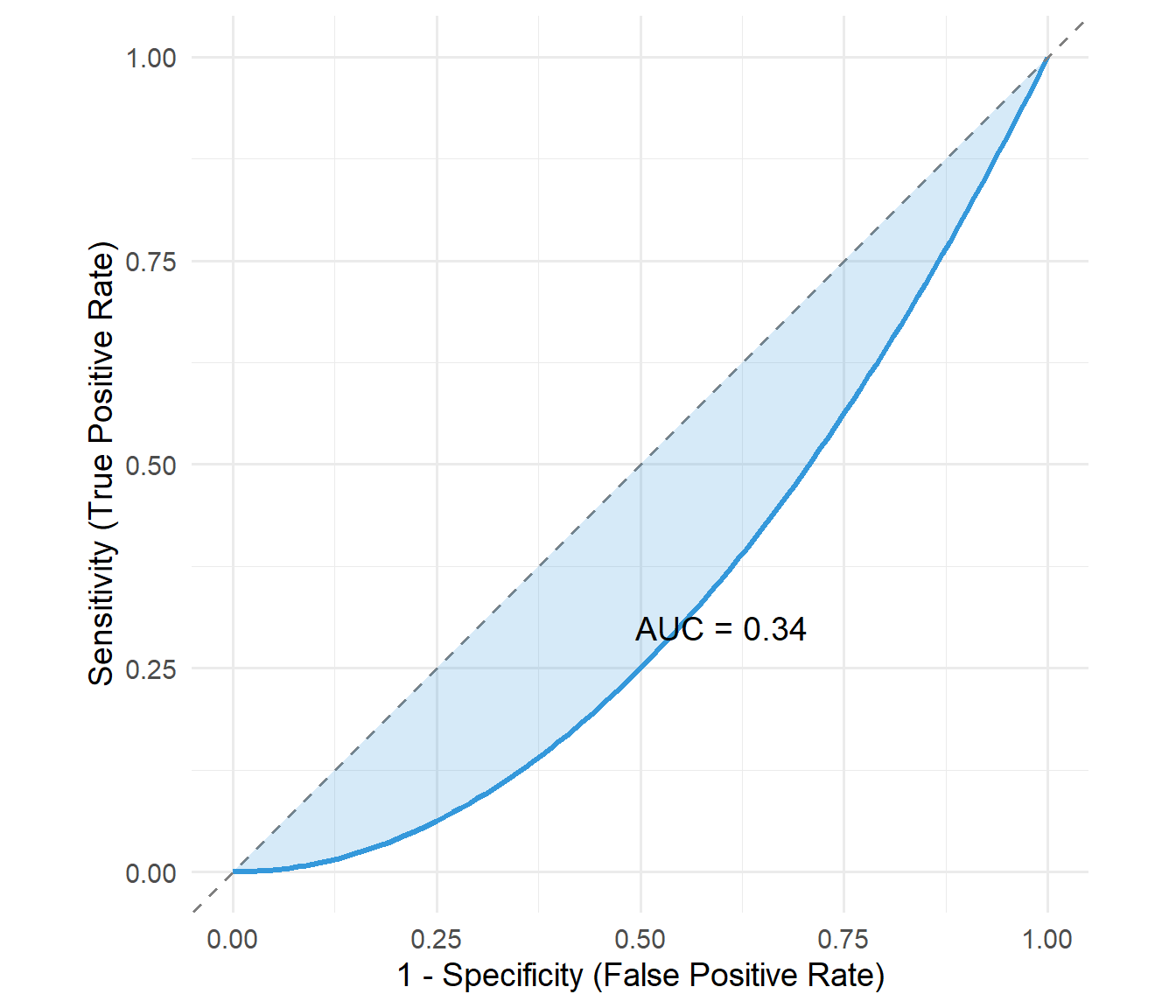
11.7 ROC Curves
The receiver operating characteristic (ROC) curve provides a way of assessing an optimal cut-off value for a test. A ROC curve plots sensitivity against (1 - specificity) at all potential cut-off points. It essentially compares the probabilities of a positive test result in those with and without disease.
The overall accuracy can be assessed by the area under the curve (AUC):
AUC = 0.5: No discrimination (test is no better than chance)
Table 11.2: PSA test results for prostate cancer detection (threshold ≥2.1 ng/ml)
True Disease Status
Prostate cancer
No prostate cancer
Total
PSA ≥2.1 ng/ml (positive)
167
508
675
PSA <2.1 ng/ml (negative)
282
1993
2275
**Total**
**449**
**2501**
**2950**
Calculating the Measures
code
# Values from the tablea <-167# True positiveb <-508# False positivec <-282# False negatived <-1993# True negativen <- a + b + c + d# Calculate measuressensitivity <- a / (a + c)specificity <- d / (b + d)ppv <- a / (a + b)npv <- d / (c + d)prevalence <- (a + c) / nlr <- sensitivity / (1- specificity)
If there is no prostate cancer, there is an 80% chance of a negative result. 20% of people will have a false positive result.
Positive Predictive Value:
\[\text{PPV} = \frac{167}{167 + 508} = 0.25\]
There is a 25% chance that if the test is positive the patient actually has prostate cancer.
Negative Predictive Value:
\[\text{NPV} = \frac{1993}{282 + 1993} = 0.88\]
There is an 88% chance, if the test is negative, that the patient does not have prostate cancer. This means there is a 12% chance of a false negative result.
Likelihood Ratio:
\[\text{LR} = \frac{0.37}{1 - 0.8} = 1.83\]
If the test is positive, the patient is 1.83 times (almost twice) as likely to have prostate cancer as not have it.
Summary of Results
code
summary_table <-tibble(Measure =c("Sensitivity", "Specificity", "Positive Predictive Value", "Negative Predictive Value", "Prevalence", "Likelihood Ratio"),Value =c(paste0(round(sensitivity *100, 1), "%"),paste0(round(specificity *100, 1), "%"),paste0(round(ppv *100, 1), "%"),paste0(round(npv *100, 1), "%"),paste0(round(prevalence *100, 1), "%"),round(lr, 2) ),Interpretation =c("37% of cancers detected","80% of non-cancers correctly identified","25% of positive tests are true cancers","88% of negative tests are truly cancer-free","15% of population has prostate cancer","Positive test ~2× more likely in cancer" ))summary_table |>kable() |>kable_styling(bootstrap_options =c("striped", "hover"))
Table 11.3: Summary of diagnostic test measures for PSA ≥2.1 ng/ml